Many VLA models today generate actions with a diffusion or flow-matching action head, and they are trained on demonstration data that is inherently multi-modal: given the same observation, different operators (or the same operator on different days) may take very different but equally valid actions. To monitor such a model during training, a common practice is to hold out a validation set, sample an action (chunk) from the policy for every validation observation, and compute its mean squared error against the ground-truth action. Another natural metric is the training objective itself evaluated on the validation set, i.e., the velocity (or noise) prediction loss.

In practice, these two metrics sometimes go in opposite directions: the action MSE keeps decreasing while the velocity loss starts to increase. Which one should we trust? In this post I’ll argue that, for a policy trained on multi-modal data, the action MSE is the misleading one, and introduce the energy score, a sample-based metric that is suitable for evaluating a stochastic policy.

A 1D toy example

Consider a 1D action $y$ whose ground-truth distribution (for some fixed observation, which we drop for brevity) has two equally likely modes:

For example, a robot can go around an obstacle either from the left ($-1$) or from the right ($+1$), but definitely not straight ahead ($0$). A flow-matching policy learns a velocity field $v_\theta(x,t)$ by minimizing

and generates an action by integrating $\frac{dx}{dt}=v_\theta(x,t)$ from a noise sample $x_0\sim\mathcal{N}(0,1)$ at $t=0$ to $t=1$.

To mimic what can happen to a model during training, consider a family of policies whose two modes are gradually pulled towards each other:

$\lambda=0$ is a perfect policy ($P_0=Q$), and $\lambda=1$ completely collapses the two modes into a single one at the mean action $0$. For each $P_\lambda$, we use the exact velocity field that generates it (which has a closed form for a Gaussian mixture), and evaluate it against the ground-truth data with two metrics:

• Velocity MSE loss: $\mathcal{L}_{\text{vel}}$ above, with $x_1$ drawn from the ground truth $Q$.
• Action MSE loss: $\mathbb{E}_{X\sim P_\lambda, Y\sim Q}(X-Y)^2$, where $X$ is a sampled action and $Y$ is the ground-truth action.

Drag the slider below to see how the two metrics change as the modes collapse. The demo also shows the energy score and a reverse KL divergence, which we will introduce later.

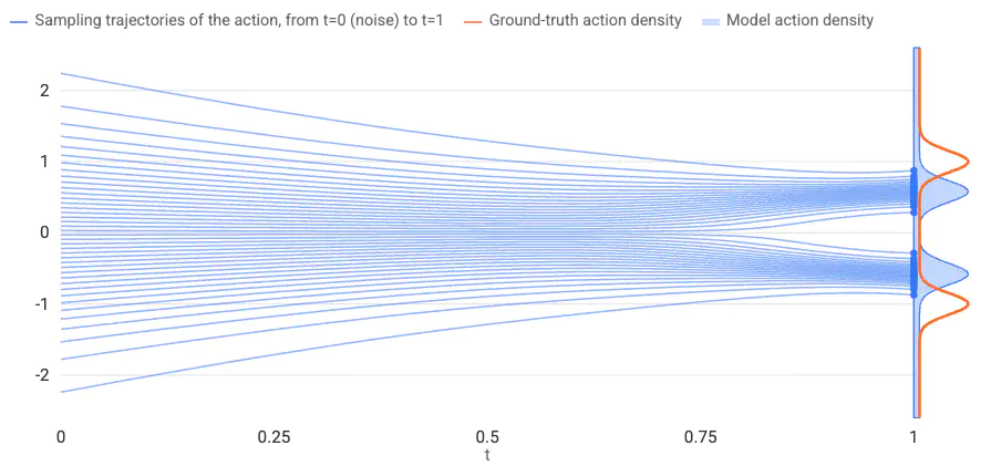
At $\lambda=0$, the sampling trajectories split into the two ground-truth modes, and the velocity loss is at its minimum. (It is not zero, because the same $x_t$ can be reached by many different $(x_0,x_1)$ pairs, so the regression target is inherently noisy.) Yet the action MSE of this perfect policy is about 2.05. As $\lambda$ increases, the action MSE decreases monotonically and is halved at $\lambda=1$, where every sample is (roughly) the invalid “go straight” action. Meanwhile, the velocity loss increases by more than 4x.

This is easy to explain. Because a sampled action $X$ and the ground-truth action $Y$ are independent given the observation,

$\text{Var}(Y)$ is fixed by the data, so the action MSE is minimized by $\text{Var}(X)=0$ and $\mathbb{E}X=\mathbb{E}Y$: a deterministic policy that always outputs the conditional mean action. A perfect policy $P=Q$ gets $2\text{Var}(Y)$, twice the error of that collapsed policy. In other words, the problem is not that the action MSE is noisy; its optimum is simply the wrong distribution. The action MSE is the right metric for a deterministic regression policy (that is what it was trained to minimize), but for a generative policy trained on multi-modal data it actively rewards mode collapse.

So why not just use the velocity loss? It is indeed a faithful metric for a single flow-matching model, but it has some limitations:

1. Its value depends on the parameterization (velocity, noise, or $x_1$ prediction), the interpolation path, and the time sampling distribution and weighting. So it cannot compare models trained with different recipes, let alone policies that are not flow-matching models (e.g., regression heads or autoregressive action tokens).
2. It evaluates the velocity field at interpolants instead of the actions that the robot actually executes. Things like the number of integration steps or other inference-time tricks are not reflected.

What we want is a metric that, like the action MSE, is computed from sampled actions, but that, unlike the action MSE, is minimized only when the sampled action distribution matches the ground-truth one. The energy score is such a metric.

The energy score

Energy distance

Let $P$ be the predicted action distribution and $Q$ the ground-truth action distribution for an observation. Draw $X,X'\overset{\text{iid}}{\sim}P$ and $Y,Y'\overset{\text{iid}}{\sim}Q$, all independent. The energy distance [1] is

where $d$ is the root mean square (RMS) distance between actions $x,y\in\mathbb{R}^D$.

Intuition. $D_E$ compares how far apart points are across the two distributions with how far apart points are within each one:

• $\mathbb{E}\,d(X,Y)$: the typical distance from a predicted action to a ground-truth action.
• $\mathbb{E}\,d(X,X')$ and $\mathbb{E}\,d(Y,Y')$: the typical spread of each distribution.

If $P=Q$, a predicted action is no farther from a ground-truth action than two ground-truth actions are from each other, so the cross term equals the within terms and $D_E=0$. Any mismatch in location, spread, or shape (for example, a missing mode) makes the cross term larger, so $D_E>0$. Formally, $D_E(P,Q)\ge 0$, with equality iff $P=Q$ (proof in the Appendix).

It’s worth noting what happens if we use the squared distance instead. By the same variance decomposition as above, $2\,\mathbb{E}\|X-Y\|^2 - \mathbb{E}\|X-X'\|^2 - \mathbb{E}\|Y-Y'\|^2 = 2\|\mathbb{E}X-\mathbb{E}Y\|^2$, which only compares the means of the two distributions. The non-squared distance is essential: it is what makes the energy distance sensitive to the full shape of a distribution.

From distance to score

We cannot evaluate $D_E$ directly: each observation has only one ground-truth action $y$, so $\mathbb{E}\,d(Y,Y')$ cannot be estimated. That term does not depend on $P$, though, so we drop it and halve the rest. This gives the energy score [2]:

The second term is constant in $P$, so minimizing the expected ES is the same as minimizing $D_E$. The minimum is reached only at $P=Q$. Compared with the action MSE, the first term is just the (non-squared) action error, and the second term is a reward for sample diversity, which cancels out the penalty that the first term puts on a well-spread, correct distribution.

In the toy example above ($D=1$, $d(x,y)=|x-y|$), the purple curve shows the expected energy score $\mathbb{E}_{y\sim Q}\,\text{ES}(P_\lambda,y)$. Unlike the action MSE, it is minimized at $\lambda=0$ and increases as the modes collapse, agreeing with the velocity loss.

Why the samples are independent

The independence assumption is about the samples, conditioned on the observation $o$; $P$ and $Q$ themselves are fixed distributions. The flow-matching policy produces a sample by integrating the learned ODE from Gaussian noise:

Given $o$ and the trained weights $\theta$, the integration is deterministic, so all of the randomness in $X$ comes from $z$.

• $X\perp Y\mid o$: $z$ is drawn fresh at inference and never sees the dataset’s ground-truth action $y$. On held-out validation data, $\theta$ was also not fit to $y$. (On training data, $\theta$ depends on $y$, so the score is optimistic, as with any in-sample metric.)
• $X\perp X'\mid o$: the $S$ samples come from $S$ independent noise draws $z_1,\ldots,z_S$.

Similar is not dependent. Training makes $P\approx Q$, but that is a statement about distributions, not about individual draws. $\theta$ learns $Q$ from other samples; a held-out $y$ is a fresh draw that $\theta$ never saw, so knowing $y$ says nothing about $X$ beyond what $o$ already does. Independence breaks only when $\theta$ was fit to that specific $y$: on training data, or when validation frames leak from training episodes. In those cases $X$ lands unusually close to $y$ and the score is optimistic.

Estimation from samples

For each observation, the model draws $S\ge 2$ samples $x_1,\ldots,x_S\sim P$, and we compare them with the single ground truth $y$:

Both terms are unbiased: the first averages over samples, and the second averages over all distinct sample pairs. Therefore $\mathbb{E}\,\widehat{\text{ES}} = \text{ES}(P,y)$. The final metric is the average of $\widehat{\text{ES}}$ over all validation observations.

A batched PyTorch implementation is only a few lines. It uses the plain Euclidean norm. Dividing the result by $\sqrt{D}$ gives the RMS version above, which only rescales the score.

import torch


def energy_score(samples, gt):
    r"""Energy score of policy samples against ground-truth actions.

    For each observation, with M samples a_1..a_M from the policy and
    ground-truth action a, the unbiased estimator is:

        ES = (1/M) * sum_i ||a_i - a||
             - 1/(2*M*(M-1)) * sum_{i != j} ||a_i - a_j||

    The returned value is the mean of ES over the batch. Lower is better.
    The norm is the (unsquared) Euclidean norm. The score is minimized only
    when the policy's action distribution matches the data distribution.

    Args:
        samples: (B, M, D) policy samples, M >= 2 per observation.
            Flatten action chunks to D = horizon * action_dim.
        gt: (B, D) ground-truth actions.

    Returns:
        Scalar tensor: energy score averaged over the batch.
    """
    M = samples.shape[1]
    acc = (samples - gt[:, None]).norm(dim=-1).mean(dim=1)
    pair = torch.cdist(samples, samples).sum(dim=(1, 2)) / (M * (M - 1))
    return (acc - 0.5 * pair).mean()

Note that torch.cdist also returns the diagonal $i=j$, but those distances are zero, so summing over all pairs equals the sum over $i\neq j$.

Relation to the reverse KL used by GEN-0

The GEN-0 release blog [3] by Generalist AI reports a reverse KL divergence alongside the validation MSE, “which better measures mode-seeking behavior”. Its purpose there is different from ours. Together with the MSE, it characterizes how a model’s samples are distributed, rather than scoring how well they match the data distribution. They found that models with both low prediction error and low reverse KL tend to perform better with supervised fine-tuning, while models with high prediction error but low reverse KL tend to be more multi-modal and benefit more from reinforcement learning. Given $M$ policy samples $\{\hat{\mathbf{a}}_m\}_{m=1}^M$ and the ground-truth action $\mathbf{a}^\star$, they define (note that $q$ is the policy and $p$ the data here, the opposite of our $P,Q$)

Plugging in the Gaussian densities (the normalizing constants cancel), the estimator becomes

Interestingly, it has the same structure as the energy score: an error term to the ground truth, plus a term that rewards diverse samples (the second term becomes more negative as the samples spread out). The difference is in how the two terms are measured. The energy score uses the same distance $d$ in both terms, and that is exactly what makes them balance so that the expected score is minimized only at $P=Q$. In the reverse KL estimator, the error term is a squared distance while the diversity term is a log-sum-exp over a Gaussian kernel with a fixed unit bandwidth. These two do not balance in general. This is not an issue when reading the reverse KL next to the MSE: since it is roughly half the MSE minus a sample-diversity bonus, the pair separates prediction error from spread, consistent with how GEN-0 interprets it. But it means that, on its own, the reverse KL is not minimized by the ground-truth distribution, and which distribution it prefers depends on the kernel bandwidth relative to the action scale.

What if we use the reverse KL for checkpoint selection?

Suppose we took the reverse KL out of its diagnostic role and used it as a single score to select checkpoints. We can check what it would prefer on the toy example. Replacing the unit bandwidth by a general $h$ (i.e., $\mathcal{N}(\cdot,h^2\mathbf{I})$ in both $q$ and $p$) and taking $M\rightarrow\infty$, the collapse level $\lambda$ that minimizes the expected reverse KL is:

This is the green dotted curve in the interactive demo above, where you can switch the bandwidth and watch its minimum (the hollow circle) move.

The toy actions have an overall standard deviation of about 1, so $h=1$ corresponds to a unit-variance kernel on normalized actions. With it, the reverse KL prefers a policy whose two modes are already partially collapsed. With a smaller bandwidth, it prefers an almost completely collapsed policy, just like the action MSE. In contrast, the energy score always prefers $\lambda=0$. It has no bandwidth to tune, and rescaling the actions simply rescales the score. Moreover, the reverse KL estimator is biased for a finite $M$ (each $\log q(\hat{\mathbf{a}}_m)$ includes the sample’s own kernel $m'=m$), whereas $\widehat{\text{ES}}$ is unbiased for any $S\ge 2$.

None of this is a problem for how GEN-0 uses the reverse KL. It is a caution against repurposing a mode-seeking diagnostic as a selection metric. If the goal is to select checkpoints or compare models by how well the sampled actions match the demonstration distribution, we want a metric whose optimum is that distribution, and the energy score is one.

Real evaluation curves

Finally, below are the validation curves of the three metrics from one of our VLA training runs with a flow-matching action head. All three metrics drop quickly in the first 10k steps, so we only show steps after that. The three metrics have different units and scales, so each curve is min–max normalized (on a log scale) over the steps shown. Thin lines are the raw values and thick lines are smoothed.

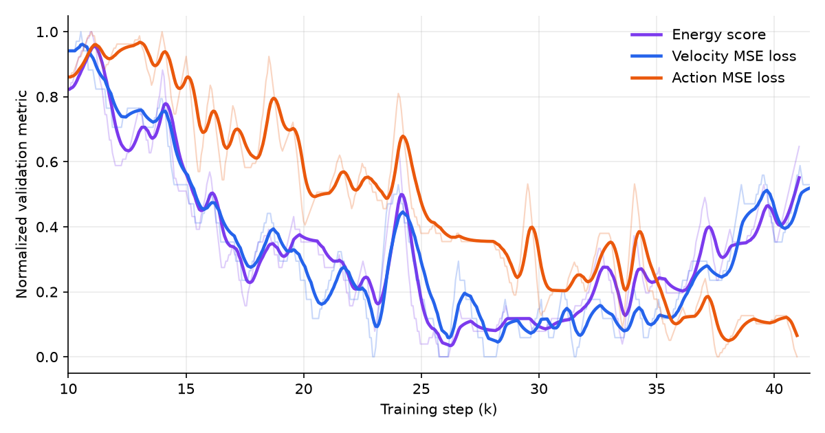
After roughly 25k steps, the velocity MSE loss and the energy score reach their minima and start to creep up, while the action MSE loss keeps decreasing until the end of training. Based on the toy example, this is the signature of the sampled action distribution starting to contract: the action MSE rewards it, while the other two metrics penalize it. If we selected the checkpoint by the action MSE, we would pick the last one, while both the velocity loss and the energy score would prefer a checkpoint around 25k–30k steps. Note that the energy score agrees with the velocity loss even though, just like the action MSE, it is computed purely from sampled actions.

To summarize: when a policy is trained on multi-modal data, don’t select checkpoints or compare models by the sampled action MSE. The velocity loss on validation data is a good sanity check within a single flow-matching model, and the energy score is a sample-based metric that works across different models and action heads.

Appendix: proof that the energy distance is non-negative

The factor $\frac{1}{\sqrt{D}}$ only rescales $D_E$, so we use $\|\cdot\|_2$. Assume $\mathbb{E}\|X\|,\mathbb{E}\|Y\|<\infty$.

Step 1: one dimension. Let $F,G$ be the CDFs of scalar $X,Y$. For any $a,b\in\mathbb{R}$, the integrand below is 1 exactly when $t$ lies between $a$ and $b$, and 0 otherwise. Its integral is therefore the length of that interval:

where the second equality holds because the square of a difference of two indicators is 1 exactly when one is 1 and the other is 0. Substituting $a=X$, $b=Y$ and taking expectations, we swap $\mathbb{E}$ and $\int$ (the integrand is non-negative). Independence of $X$ and $Y$ then factors each term:

and likewise for the second term, which gives $G(t)\big(1-F(t)\big)$. Hence

Setting $G=F$ (for $X,X'$) and $F=G$ (for $Y,Y'$) in the same formula gives

Therefore

with equality iff $F=G$.

Step 2: $D$ dimensions. The idea is to write the $D$-dimensional norm as an average of 1D absolute values, then apply Step 1 to each one.

(a) The norm as an average of projections. Let $\theta$ be a random unit vector, uniform on the sphere, and define $f(x)=\mathbb{E}_\theta|\theta^\top x|$, the average length of the “shadow” of $x$ on a random line. This function has two properties:

• Rotation invariant: for any rotation $R$, $f(Rx)=\mathbb{E}_\theta|(R^\top\theta)^\top x| = f(x)$, because $R^\top\theta$ is also uniform on the sphere. So $f(x)$ depends only on $\|x\|$.
• Scales linearly: $f(cx)=c\,f(x)$ for $c\ge 0$.

Hence $f(x)=f(e)\,\|x\|$ for any unit vector $e$, and

For example, in $D=2$, $f(e)=\mathbb{E}|\cos\phi| = 2/\pi$, so $\|x\|=\frac{\pi}{2}\mathbb{E}_\theta|\theta^\top x|$.

(b) Apply it to each term. Write $X_\theta=\theta^\top X$ and $Y_\theta=\theta^\top Y$. These are scalars with 1D distributions $P_\theta$ and $Q_\theta$, and they are still independent. Take $x=X-Y$, so that $\theta^\top x = X_\theta - Y_\theta$. Taking $\mathbb{E}$ over $X,Y$ and swapping it with $\mathbb{E}_\theta$ (the integrand is non-negative):

In the same way, $\mathbb{E}\|X-X'\| = k_D\,\mathbb{E}_\theta\,\mathbb{E}|X_\theta-X'_\theta|$ and $\mathbb{E}\|Y-Y'\| = k_D\,\mathbb{E}_\theta\,\mathbb{E}|Y_\theta-Y'_\theta|$.

(c) Combine. Substituting into the definition of $D_E$:

The bracket is exactly the 1D energy distance between $P_\theta$ and $Q_\theta$, which is $\ge 0$ by Step 1. An average of non-negative numbers is non-negative, so $D_E(P,Q)\ge 0$.

(d) Equality. If $D_E(P,Q)=0$, then $D_E(P_\theta,Q_\theta)=0$ for almost every $\theta$, so $P_\theta=Q_\theta$ by Step 1. A distribution is uniquely determined by its 1D projections (Cramér–Wold), so $P=Q$. $\blacksquare$

References

[1] G. J. Székely and M. L. Rizzo. Energy statistics: A class of statistics based on distances. Journal of Statistical Planning and Inference, 143(8):1249–1272, 2013.

[2] T. Gneiting and A. E. Raftery. Strictly proper scoring rules, prediction, and estimation. Journal of the American Statistical Association, 102(477):359–378, 2007.

[3] Generalist AI Team. GEN-0: Embodied foundation models that scale with physical interaction. Generalist AI Blog, November 4, 2025. https://generalistai.com/blog/gen-0