Learning the Q value of multi-step actions

Assume that we have a policy $\pi(a_{0:k-1}|s_0)$ that is able to output a variable length $k$ of actions given any state $s_0$. We define a Q function $Q(s_0,a_{0:k-1})$ which computes the state-action value of any action sequence $a_0,a_1,\ldots,a_{k-1}$ given $s_0$. The intuitive meaning of this quantity is: what expected future return will we get, if starting from $s_0$, we take actions $a_0,a_1,\ldots,a_{k-1}$ regardless of the future states in the following $k$ steps, after which we follow our policy $\pi$? In fact, our $k$-step action sequence is open-loop because it doesn’t depend on the environment feedback in the next $k$ steps.

We can use the Bellman equation to learn $Q(s_0,a_{0:k-1})$ from the data of a memory (e.g. a replay buffer or a search tree). The bootstrapping target for $Q(s_0,a_{0:k-1})$ is defined as

$$ \mathcal{T}^{\pi} Q(s_0,a_{0:k-1}) = \sum_{i=0}^{k-1}\gamma^i r_i + \gamma^k \mathbb{E}_{s_k\sim P(\cdot|s_0,a_{0:k-1})}\mathbb{E}_{a_{k:k+k'-1}\sim \pi(\cdot|s_k)}Q(s_k,a_{k:k+k'-1}), $$

where $P(s_k|s_0,a_{0:k-1})$ is the environment transition probability. In practice, each time we sample a $k$-step transition $s_0,a_{0:k-1},s_k$ from the memory, sample a new sequence of actions $a_{k:k+k'-1}\sim \pi(\cdot|s_k)$ with the current policy, and use $\sum_{i=0}^{k-1}\gamma^i r_i + \gamma^k Q(s_k,a_{k:k+k'-1})$ as a point estimate of the above target to fit $Q(s_0,a_{0:k-1})$. So the key question is: whether the empirical frequency of $s_k$ (from the memory) correctly matches the theoretical distribution of $s_k$ after we executes $a_{0:k-1}$ in an open loop manner at $s_0$?

The answer is not always, and it depends on how the transition $s_0,a_{0:k-1},s_k$ is obtained from the memory (e.g. replay buffer or search tree). In a usual case, the action sequence $a_{0:k-1}$ might come from stitching two action sequence outputs during rollout, as the example below shows.

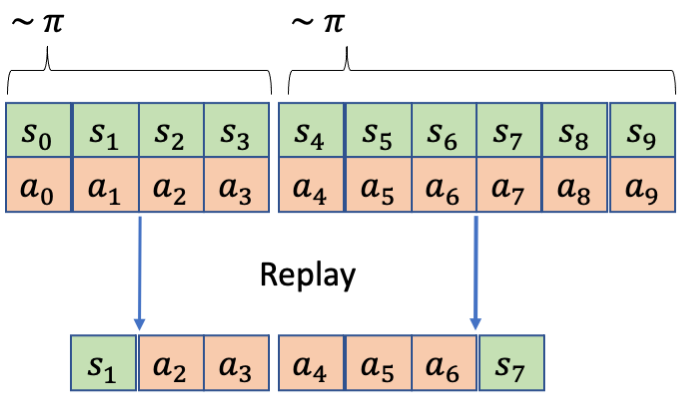
Here, the replayed transition $s_1,a_{2:6},s_7$ actually spans over two rollout policy samplings. This might cause issues for learning the state-action value in some MDPs.

Deterministic environment

For a deterministic environment, it’s completely fine to learn $Q(s_0,a_{0:k-1})$ by arbitrarily stitching together temporally contiguous $a_{0:k-1}$ from a memory, even though these actions were not generated in one shot (i.e., generated once for all at $s_0$). The reason is that given $s_0$ and any subsequence $a_{0:m}(m\le k-1)$, $s_{m+1}$ is uniquely determined in a deterministic environment. So the final state $s_k$ correctly reflects the transition destination state with a probability of 1.

MCTS and MuZero

Tree search algorithms such as MCTS and MuZero will estimate the Q values of actions at a root node by expanding the search tree for multiple (learned) environment simulations. This estimation essentially uses $$\sum_{i=0}^{k-1}\gamma^i r_i + \gamma^k Q(s_k,a_k)$$ to determine the likelihood of choosing $a_0$ at $s_0$ compared to other actions. Note that in this case, $a_{0:k-1}$ stitches together multiple actions which are sampled one by one during rollout. As discussed above, MCTS is applicable to deterministic environments.

Stochastic environment

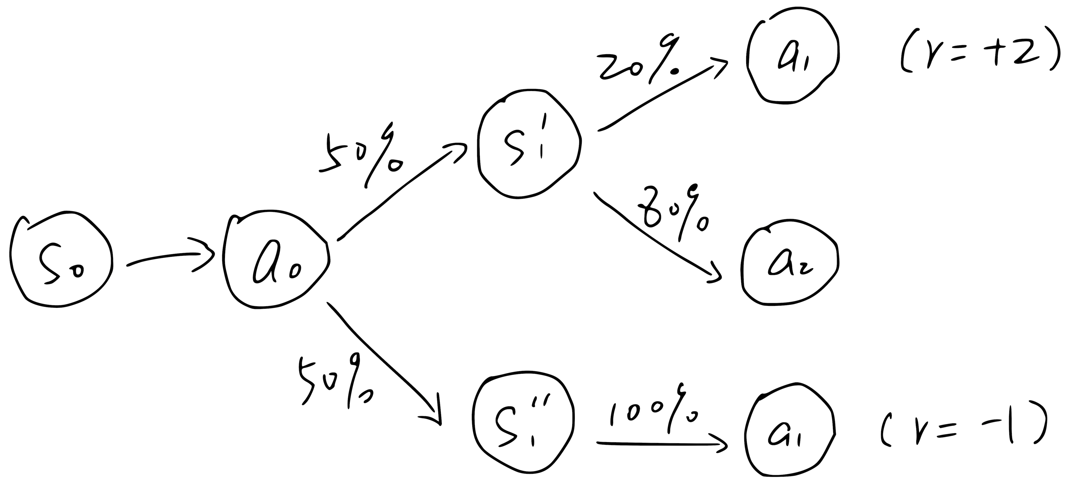
However, in a stochastic environment, arbitrarily stitching together contiguous actions will have issues. To see this, consider the example above, where $a_1$ can be generated at two different states $s_1'$ (prob of 0.2) and $s_1''$ (prob of 1), where these two states are valid stochastic successors to $(s_0,a_0)$ with a chance of 0.5. We assume that the episode always starts with $s_0$ and ends after either $s_1'$ or $s_1''$ (suppose the end state is denoted by $s_2$).

By our definition, $Q(s_0,a_{0:1})$ (the state-action value of taking $a_0$ and then $a_1$ starting from $s_0$) should be $0.5\times 2 - 0.5\times 1=0.5$. Note that when we compute this value, we should not look at the action distribution at $s_1'$ or $s_1''$. Even though $a_1$ has only a prob of 0.2 at $s_1'$, we always take it after $a_0$.

Now suppose all data in the memory are generated step by step. When using TD learning to estimate $Q(s_0,a_0,a_1)$, we sample either $(s_0,a_0,s_1',a_1,s_2)$ or $(s_0,a_0,s_1'',a_1,s_2)$ from the memory. The problem is, the second transition appears 4x more frequently than the first one! Thus the learned $Q(s_0,a_0,a_1)$ will be $\frac{5}{6} \times -1 + \frac{1}{6}\times 2=-0.5$. This is completely wrong given the correct value of 0.5.

So what happened? In this case, we can only learn the correlation between $(s_0,a_0,a_1)$ and $Q(s_0,a_0,a_1)$ but not their causal relationship (i.e., what expected return we will get if taking $a_0,a_1$ staring from $s_0$?).

MCTS and MuZero

It is well known that MCTS-based algorithms will have similar issues in stochastic environments.

How to avoid the causal confusion

For a policy $\pi(a_{0:k-1}|s_0)$ that is able to output a variable length $k$ of actions given any state $s_0$, in general we need to honor the action sequence boundary when sampling from the memory for TD learning. That is to say, in the first figure, we can only sample subsequences within $(a_0,a_3)$ or $(a_4,a_9)$, but not across the boundary $a_3|a_4$.

(However, this solution is not applicable to MCTS or MuZero because when expanding a root node, they always take actions at every tree node and stitch together actions along a tree path.)