On Sim2Real transfer in Robotics （Part 2/3)

Physics Sim2Real Gap (continued)

System identification errors

Controller in the loop of policy control

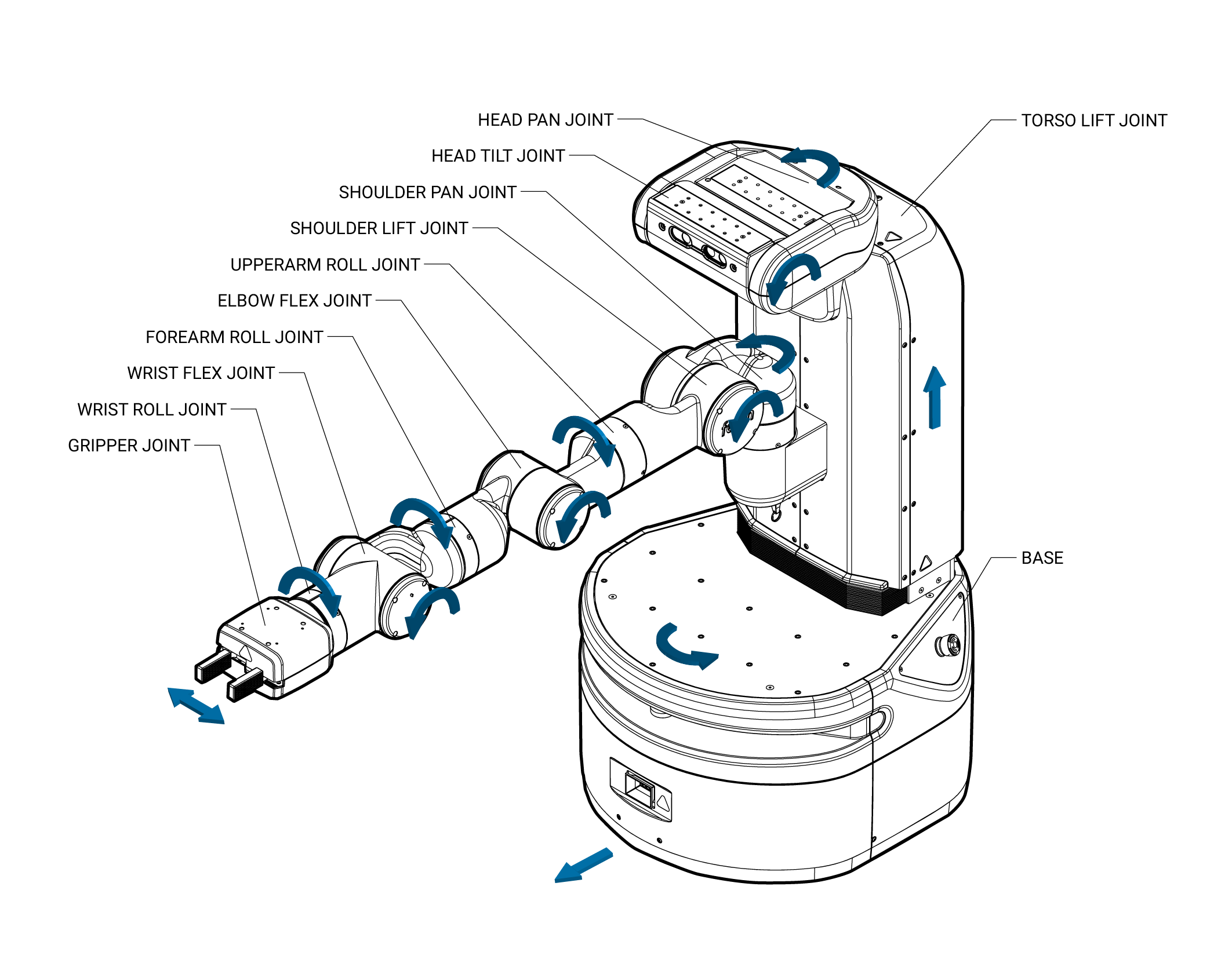
A robot typically consists of multiple actuators such as gear motors, each tasked with moving one or more joints. Joints serve as connections between different parts of the robot, allowing it to move in different ways by applying specific forces to its actuators. This dynamic interplay between actuators and joints allows us to view a robot as a complex dynamical system.

Fetch Robot joints (https://docs.fetchrobotics.com/robot_hardware.html)

The goal of system identification is to replicate the input-output behavior of a dynamical system accurately. In the realm of simulation, this translates to ensuring that we precisely model the robotic system to replicate its behavior.

The input-output behavior can be represented as a mapping from control to force. This mapping is called a controller. Typically, a physical robot supports multiple control spaces and we can select one based on our specific task requirements. For instance, the control could be based on joint position, joint velocity, or even joint acceleration. To simplify matters, let’s assume each joint is 1D, meaning that its position is represented by a scalar, and it can only rotate, slide, or extend within a 1D range. Thus the controller is formally noted as $a_i \rightarrow f_i$, where $a_i$ is the target control of the $i$-th joint and $f_i$ is the output force by the actuator in response to the control. The force will then be translated to current driving the corresponding actuator. The generation of force in response to the control is governed by algorithms which we will discuss later.

It’s crucial to understand that $a_i$ is the “target” control and might not be equal to the actual joint state after applying the force. In the physical world, there is no guarantee that this target (whether it’s a joint’s position, velocity, or acceleration) will be achieved before the next control signal is dispatched to the controller. Imagine a scenario where the controller operates at a frequency of 10Hz, allotting just 0.1 seconds for each cycle. In such a tight window, striving for the target state of each joint becomes challenging, primarily because it takes time for the applied force to the actuator to take effect and for the complex dynamical system to stabilize. If the target is missed, the show must go on! The controller receives an updated control target and proceeds to output revised forces to the actuators.

This wild scenario is in stark contrast to certain “toy” simulated robots. For example, when I first got in touch with learning-based robotics, I used to run lots of RL experiments in OpenAI’s classic Fetch robot environment.

Simulated Fetch in OpenAI gym

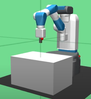The dynamical system of this robot is so simplified that it is assumed that a MoCap body of MuJoCo is attached to the gripper so that it is guaranteed that the gripper will move to any $(x,y,z)$ position in the control space for each control step! In other words, the control target will always be met at every step. This assumption, of course creates a huge physics Sim2Real gap for deploying such a simulation-trained policy on a real Fetch robot, simply because the real world dynamics does not have the “MoCap property” (we cannot freeze the time while letting the controller to stabilize at the target control).

Normally, an NN policy that outputs $a_i$ has to learn to factor in the controller dynamics. It outputs the action based on a prediction of how the controller will respond to that target control. Thus if the policy is deployed to a real robot with a mismatched controller dynamics, the policy will fail due to an incorrect dynamics expectation.

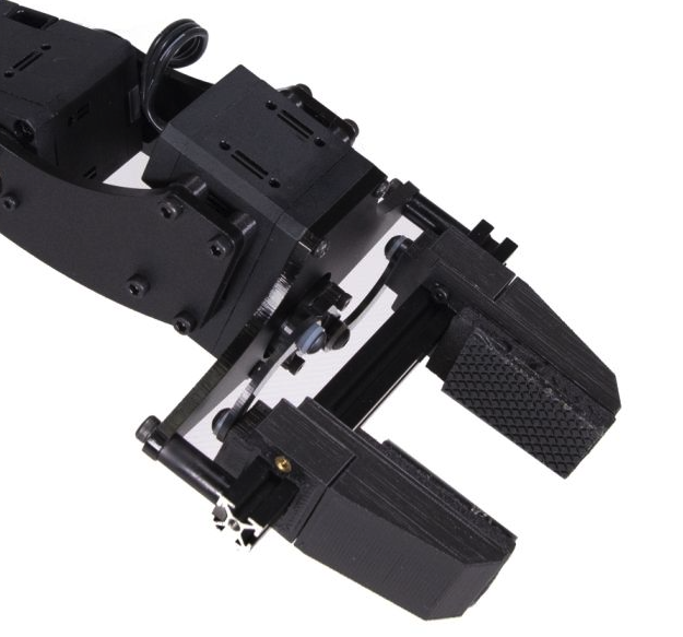
Why not aim to minimize system identification errors? We seek to ensure our robot hardware achieves high precision while the simulated controller model mirrors the real one exactly. However, achieving this is no easy feat. Firstly, while there are industry-grade robots renowned for their precision, they often come with a hefty price tag and aren’t widely adopted in daily scenes. Secondly, for certain robots, accurately mirroring their controllers poses a challenge due to limited capacities of the simulator or limited simulation effort. Take, for instance, the Widowx250s arm, which features a unique gripper design. In this setup, both fingers are driven by a single motor. As the motor rotates, it equally pushes and pulls both fingers along the supporting structure. If we use MuJoCo to simulate this robot arm, it is not straightforward to model this gripper dynamical system, and some approximation is needed.

Widowx250s gripper

SISO controller

Before we answer how to get around system identification errors in the presence of cheap robot hardware and an imperfect simulator, we need to first talk about common controller algorithms.

Recall that the general objective of a controller is:

$min_{\mathbf{f}}\frac{1}{2}\Vert \mathcal{A}(\mathbf{f},\mathbf{s};\Delta t) - \mathbf{a} \Vert^2,$

subject to the time constraint of a control interval $\Delta t$. Here we assume the robot dynamical system is a function, denoted by $\mathcal{A}$, of the force vector $\mathbf{f}$ output by actuators and the current joint state $\mathbf{s}$. Let’s say we are doing position control and $\mathbf{a}$ stands for the target joint positions. $\mathcal{A}$’s output is the actual joint positions at the end of the control interval. Alternatively, $\mathbf{a}$ can be other joint state such as velocity, acceleration, etc.

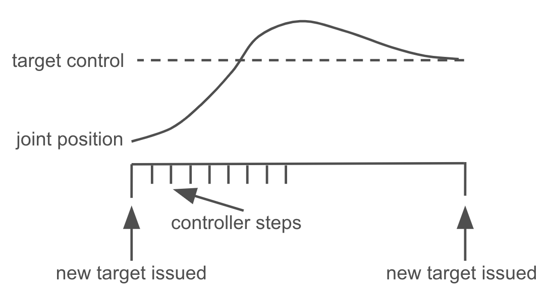
The optimal value of the objective above is called the tracking error. It basically indicates how closely a sequence of control targets can be tracked by a controller. A zero tracking error means that given a control frequency, the controller can exactly realize every control target output by an NN policy. In this case, the policy will not have to learn the robot dynamics. It is just equivalent to having a MoCap body for the joints.

Illustration of tracking errors. 'x' marks a new control target.

If $\mathcal{A}$ is known, then we can just do gradient descent and get an “optimal” controller. However, $\mathcal{A}$ is often unknown (due to interaction with the environment) and we have to rely on simple approximation solutions in practice.

A common simplification often used is assuming independence among joints. Rather than employing a multi-input multi-output (MIMO) controller, we can opt for assigning a single-input single-output (SISO) controller to each joint, allowing the controllers to operate independently.

$min_{f_i}\frac{1}{2}(\mathcal{A}(f_i,s_i;\frac{\Delta t}{N}) - a_i )^2.$

Although SISO control may sound simplistic at first glance, it can actually wield significant power and is widely embraced in robotics applications. The reason is that SISO control can be performed closed-loop in an adaptive manner. Given a control interval of $\Delta t$, we can divide it into multiple $N$ small segments, where at each segment of length $\frac{\Delta t}{N}$ the controller has an opportunity to adjust its output given the current joint position and the target control. Its joint position might be impacted by other joints due to physical constraints, but as long as the controller can adjust its output frequently, it is still able to reach the target. It is this flexibility that makes SISO controllers practical even though each controller is unaware of others when making a decision.

Closed-loop SISO controller

In the following discussion, our focus will be on SISO controllers.

P, I, PI, and PID controllers

P. A Proportional (P) controller is just like doing one-step gradient descent. Denote the objective loss for the $i$-th controller as $L_i$. According to the chain rule, the gradient can be computed as

$\frac{\partial L_i}{\partial f_i}=\frac{\partial L_i}{\partial \mathcal{A}_i}\frac{\partial \mathcal{A}_i}{\partial f_i}=(\mathcal{A}_i-a_i)\frac{\partial\mathcal{A}_i}{\partial f_i}$.

Because we do not know $\mathcal{A}_i$, we can simply assume a constant value for $\frac{\partial\mathcal{A}_i}{\partial f_i}$ as 1 and $\mathcal{A}(f_i,s_i;\frac{\Delta t}{N})\approx a_i^t$ (current joint position) because of a very small $\frac{\Delta t}{N}$. Also assuming the optimization starts with $f_i=0$, then the output of the P controller after one step of gradient descent is:

$f_i^*=0 - (a_i^t-a_i)\cdot Kp = (a_i-a_i^t)\cdot Kp.$

The gradient descent step size in this context is called the Kp parameter, a constant determining how responsive a P controller is to a target control. The intuition of a P controller is very simple: each time the controller compares the target control with the current joint position, and sets the output force linearly proportional to the difference.

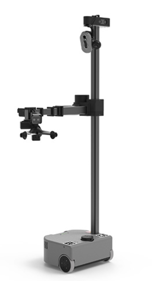
A well-known issue with P controller is that it might generate a steady-state error for each joint. For example, imagine there is a joint can slide up and down to change the height of the robot arm, something similar to what Stretch 3 has.

Stretch 3 by Hello Robot

With P control, if we set the control target to be a height of $h$, the actual height $h’$ will be always less than $h$. Why? Because P control needs $h-h’>0$ to generate a force to offset the arm weight, otherwise the arm would just fall until there is enough force generated. This steady-state error $h-h’$ is the minimal tracking error this joint could get using a P controller.

I. An Integral (I) controller has a very similar formulation with a P controller, except that it uses an accumulated error to compute the force:

$f_i^*=\int_0^t (a_i-a_i^{t’})d{t’} \cdot Ki$

This can eliminate the steady-state error, because the force will keep increasing whenever there is non-zero error being accumulated, until the error becomes zero. However, this behavior also easily leads to a phenomenon called overshooting, where the joint state goes up and down until it finally stabilizes at the control target after some time. Thus although an I controller can guarantee a zero-tracking error eventually, in practice we might have an enough large control interval for the controller to completely settle down.

PI. We can blend a P controller with an I controller to minimize steady-state error with less overshooting.

$f_i^*= (a_i-a_i^t)\cdot Kp + \int_0^t (a_i-a_i^{t’})d{t’} \cdot Ki.$

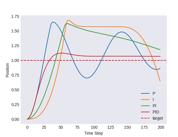
PID. A Proportional-Integral-Derivative (PID) controller adds a derivative term on top of a PI controller, to solve the overshooting issue. A D controller predicts future error based on its current trend, enabling it to anticipate and counteract potential overshoots or undershoots in the system’s response. The current rate of error changing is computed as $\frac{d (a_i-a_i^t)}{dt}$. If the rate is negative, it means that the joint state is moving in the increasing direction, and we should decrease the force to reduce overshooting. If the rate is positive, we should increase the force to reduce undershooting.

$f_i^*= (a_i-a_i^t)\cdot Kp + \int_0^t (a_i-a_i^{t’})d{t’} \cdot Ki + \frac{d (a_i-a_i^t)}{dt} \cdot Kd.$

Step response curves of different controllers

For a very good tutorial on PID controller, I suggest the readers taking a look at this video.

How to close the Sim2Real gap related to system identification errors

From the above discussions, we can see that there are at least two ways to close the Sim2Real gap related to system identification errors:

• Avoid any system identification error at all. As mentioned earlier, this requires the robot hardware to achieve high precision while the simulated controller model mirrors the real controller model exactly. If this can be achieved, then even if there is a non-zero tracking error at the end of each control interval, that error will be very similar in simulation and in real. In this case, steady-state error is not a big issue and the policy behaviors learned in simulation can be successfully transferred to real.
• Always use a PID controller to achieve nearly a zero-tracking error both in sim and in real. Suppose this is feasible, then it does not matter what the joint state trajectory looks like. There are thousands ways of approaching the target in either sim or real, but as long as the tracking error is zero, the policy will observe the same robot state for the next decision.

So how to let a PID controller achieve an almost zero tracking error? There are mainly four key factors:

1. tune the PID parameters to match the real ones,
2. use a profiling technique,
3. make sure the difference between the target control output by the policy and the current joint state is small, and
4. choose a large enough control interval so that PID control has enough time to settle down at the target.

For 1), it seems easy at first glance since we should be able to just look at the manual of a physical robot, find its PID parameters, and set the same values in our simulator. However, sometimes the implicit scales of PID parameters might not be consistent between real and sim. The same number of “50” might mean different values.

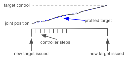
For 2), a profiler can set some gradually and smoothly changing intermediate control targets within the control interval, and guide the controller generate smaller forces. This helps reduce overshooting and minimize the tracking error.

Linear profiling

For 3), we can select a conservative action space for the policy so that a new action can only be in a small neighborhood of the current joint state. This usually results in a slow moving robot and a longer time horizon (and thus a more difficult RL problem).

For 4), if we don’t need a quickly responsive robot or high-precision robot skills, we can increase the control interval (e.g., from 10Hz to 2Hz). This makes sure the joints move to the desired state completely, before the next control target is issued for the controller. This is the main cause for some robot demos where we see regular pauses of robot movement.

Finally, what is the consequence of Sim2Real transferring a policy without properly addressing the system identification errors?

Summary

We have talked about some major possible physics Sim2Real gaps and proposed various methods to close them. In the next article, we will look further into the vision Sim2Real gap, which is another great challenge of transferring a vision-based policy from simulation to the real world.